Group by and Pivot by: create your own reports, using formulas that are updated automatically, and see when a PivotTable might still be the better option.
FAQ — What does this article answer?
Q: What do GROUPBY and PIVOTBY actually do?
A: Each one can turn a table into a summary report using just one formula. The GROUPBY function will give you one row for each group, which is like a one-dimensional PivotTable. The PIVOTBY function will create a table with two columns, one down the side and the other across the top. You can use one formula to calculate both the total and sort, and filter the data. The formula will refresh automatically when the source changes.
Q: How is this different from SUMIFS?
A: The function SUMIFS can be used to calculate the sum of a cell, but it needs a list of labels that it can use to do this. GROUPBY finds the different groups and returns the whole report as a spilled range. A SUMIFS report is a grid of formulas that you need to maintain, but a GROUPBY report is a single formula that does all the work for you.
Q: What is the difference between PIVOTBY and a PivotTable?
A: A PivotTable is an interactive object that you build by dragging fields and refreshing by hand. The PIVOTBY formula recalculates live and its result can be used in other formulas. It is part of the grid and can be tracked in version control. It doesn't have the same interactive features as a PivotTable, like slicers, drill-down, expand and collapse.
Q: Is there a way to sort and filter without using the SORT and FILTER functions?
A: Yes. Both functions take a sort_order argument (a signed column index) and a filter_array argument (a boolean column). So sorting and choosing rows is part of the report definition, not something separate.
Q: Which version of Excel have these functions?
A: You can use GROUPBY and PIVOTBY in the Microsoft 365 Current Channel (Windows and Mac) and in Excel for the web, following their general release in late 2024. They are not included in any permanent licence. This applies to Excel 2016, 2019 and 2021, and also Excel 2024. In those versions, the formula returns #NAME?.
Q: My colleagues have a licence that never expires. What should I use instead?
A: To sum up, if you want something simple, try using UNIQUE together with SUMIFS, as this is similar to GROUPBY. For a 2D matrix, a PivotTable is the sensible choice. Part 7 gives the exact patterns.
For twenty years, when people wanted to summarise a table in Excel, they had two options. They could either build a PivotTable by hand, or they could put together a grid of SUMIFS formulas against a list of labels that they had prepared in advance. Both of these options work. They are both also weak because they don't look after themselves. A PivotTable must be updated; a SUMIFS report stops working as soon as a new category appears that no one thought to add a row for.
The GROUPBY and PIVOTBY functions remove this problem. They are similar to other functions like FILTER, SORT and UNIQUE because they all work in the same way. They all return a report that is a whole grid, and it recalculates as soon as the data underneath it changes. This article is not so much about two functions as it is about a change in how reports are made. It also looks at where that change stops and when a PivotTable is still the right tool for the job.
Part 1: There are three ways to summarise a table.
It helps to see the three approaches next to each other, because each solves the previous one's main problem.
| Approach | How the report is built | The catch |
|---|---|---|
| Manual PivotTable | Drag fields into place, refresh after every change | Interactive, but static between refreshes |
SUMIFS grid |
Prepare a label list, write one formula per cell | Silently omits any group you did not list |
GROUPBY / PIVOTBY |
One formula finds the groups and returns the whole report | Requires Microsoft 365 |
This article is all about the third row. The point is not that it makes the other two redundant, it is not. But formula-native aggregation is now a key part of the worksheet. A report can be a value that other formulas consume, rather than an object stuck in a corner of a sheet. This one change is what makes the modern approach worth learning, and it is also the main point that is discussed in Part 6.
Part 2: The data we are working with
Every example below uses the same table, defined as an Excel table named Sales.
| Region | Category | Quarter | Amount | Units |
|---|---|---|---|---|
| North | Hardware | Q1 | 12,400 | 62 |
| North | Software | Q1 | 8,900 | 45 |
| South | Hardware | Q1 | 6,200 | 31 |
| South | Services | Q2 | 9,750 | 18 |
| North | Hardware | Q2 | 15,300 | 74 |
| East | Software | Q2 | 11,100 | 56 |
| South | Software | Q1 | 4,600 | 22 |
| East | Hardware | Q2 | 7,800 | 39 |
| North | Services | Q2 | 5,400 | 12 |
| East | Services | Q1 | 3,300 | 8 |
The total amount is 84,750. Remember this figure: every summary in this article refers back to it.
💡 Tip: Make the data into a table using the shortcut 'Ctrl+T' before you start. Structured references such as Sales[ Amount] then move with the columns, and the report automatically takes in new rows as they are added. The reasoning is set out in Why every dataset should be an Excel table.
Part 3: GROUPBY — one dimension, aggregated
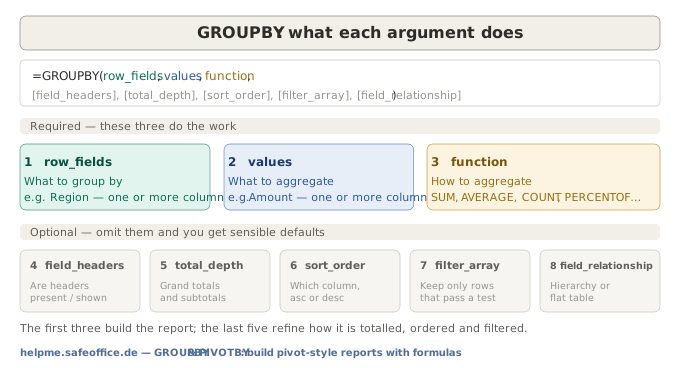
The signature has three required arguments and five optional ones:
=GROUPBY(row_fields, values, function, [field_headers], [total_depth], [sort_order], [filter_array], [field_relationship])| Argument | Required | Purpose | Default |
|---|---|---|---|
row_fields |
Yes | The column, or columns, to group by. These become the row labels. | — |
values |
Yes | The column, or columns, to aggregate. | — |
function |
Yes | How to aggregate: SUM, AVERAGE, COUNT, MAX, MIN, PERCENTOF, or a custom LAMBDA. |
— |
field_headers |
No | Whether the source has headers and whether to display them. | Automatic |
total_depth |
No | 0 no totals, 1 grand total, 2 grand total plus subtotals. A negative value places totals at the top. |
1 |
sort_order |
No | A signed column index to sort by: positive ascending, negative descending. | Source order |
filter_array |
No | A boolean column the same height as the data; TRUE keeps the row. |
All rows |
field_relationship |
No | With several row_fields: 0 hierarchy or 1 table. |
0 |
The simplest form
Total the Amount column by Region:
=GROUPBY(Sales[Region], Sales[Amount], SUM)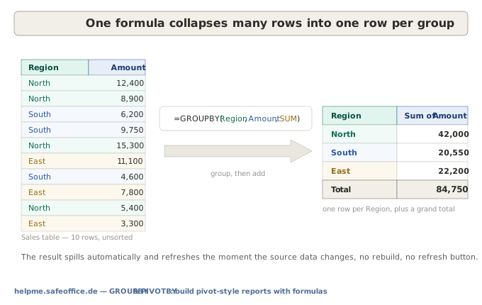
There are three things to note. The function found the three regions on its own. You never typed "North", "South" or "East". It added a grand total without being asked, because the number of levels is automatically set to 1. The result is a spilled range. If you add a fourth region to the table tomorrow, a fourth row will appear in the report immediately, with no formula to edit.
Choosing how to aggregate
The third argument is a function that is passed by name and without brackets. Excel recognises the usual calculations such as SUM, AVERAGE, COUNT, COUNTA, MAX, MIN, PRODUCT, MEDIAN, STDEV.S and VAR.S. It also recognises two more specific to this family:
PERCENTOFexpresses each group as a percentage of the whole.- A custom
LAMBDAlets you define any aggregation Excel does not provide.
To show each region's share of turnover:
=GROUPBY(Sales[Region], Sales[Amount], PERCENTOF)This returns North 49.6%, East 26.2% and South 24.2%. This is the same as a PivotTable's "% of grand total" would give, in one formula.
If you want to report more than one figure at once, either pass several value columns or stack several functions with HSTACK:
=GROUPBY(Sales[Region], Sales[[Amount]:[Units]], SUM)     ' sum of Amount and of Units, side by side
=GROUPBY(Sales[Region], Sales[Amount], HSTACK(SUM, AVERAGE))   ' total and average of Amount
The LAMBDA route is important for the argument in Part 1. Because the aggregation is a function, a report can apply logic that a PivotTable's fixed value-field menu cannot express, for example, a weighted average, a trimmed mean, or a bespoke margin calculation. If you haven't written a LAMBDA before, check out the article. LET and LAMBDA: cleaner, reusable formulas.
Totals and subtotals
The total_depth argument controls the totals. When there's only one grouping column, you can choose between 0 (a simple list, which is useful when the report is used with another formula) and 1 (the usual grand total). Subtotals, here total_depth is two, are really useful when you group by more than one field:
=GROUPBY(Sales[[Region]:[Category]], Sales[Amount], SUM, , 2)This groups things together based on where they are located and the category they fall into. It also adds up the total for each category and then adds them all together at the bottom. The empty argument before the 2 leaves field_headers at its default; the positions of the commas matter, exactly as they do in any Excel function.
Part 4: Sorting and filtering inside the formula
Sort the report
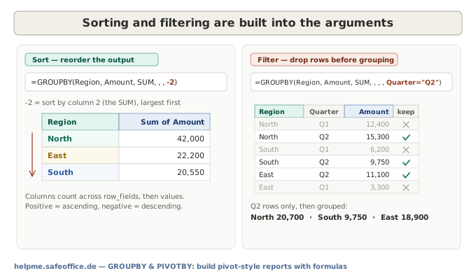
You can use a signed column index with the sort_order function. The columns are counted from left to right. First, the row_fields are counted, then the values. So in our one-group, one-value report, column 1 is Region and column 2 is the total. To sort by the total, largest first:
=GROUPBY(Sales[Region], Sales[Amount], SUM, , , -2)The result is North, East, South. If you put a positive 2 in, it will sort smallest first. The two empty arguments skip field_headers and total_depth, so both stay at their usual settings.
💡 Tip: The most common mistake people make when sorting is counting from column A of the sheet rather than from the first column of the report. Only count the columns that the function returns.
Sort the information before you put it into groups.
The filter_array is a Boolean column, which means it can only be true or false. It has the same height as the source and is evaluated before the grouping happens. To sum up the second quarter:
=GROUPBY(Sales[Region], Sales[Amount], SUM, , , , Sales[Quarter]="Q2")If you put Sales[Quarter]="Q2", you'll get a column of TRUE and FALSE values. The rows that are FALSE will be ignored, and the rest of the rows will be put into groups like normal. The report, which is only for the second quarter, says that the north is 20,700, the south is 9,750, and the east is 18,900. Because the test is an ordinary Excel expression, you can combine conditions with * for AND and + for OR, just like in FILTER. You can find all the information about Boolean criteria arrays in [Dynamic arrays with FILTER, SORT, UNIQUE and SEQUENCE].(/index.php?page=public/en/dynamic-arrays-with-FILTER-SORT-UNIQUE-SEQUENCE).
Part 5: PIVOTBY — two dimensions at once
Where GROUPBY summarises down one axis, PIVOTBY cross-tabulates two. It adds a col_fields argument and a matching pair of total and sort arguments for the column axis.
=PIVOTBY(row_fields, col_fields, values, function, [field_headers], [row_total_depth], [row_sort_order], [col_total_depth], [col_sort_order], [filter_array], [relative_to])| Argument | Required | Purpose |
|---|---|---|
row_fields |
Yes | The column, or columns, down the side |
col_fields |
Yes | The column, or columns, across the top |
values |
Yes | The column, or columns, aggregated in the body |
function |
Yes | How to aggregate |
field_headers |
No | Whether headers are present and shown |
row_total_depth |
No | Totals for the row axis (as total_depth in GROUPBY) |
row_sort_order |
No | Signed column index for sorting rows |
col_total_depth |
No | Totals for the column axis |
col_sort_order |
No | Signed index for sorting columns |
filter_array |
No | A boolean column applied before pivoting |
relative_to |
No | The denominator for PERCENTOF: 0 column total, 1 row total, 2 grand total (and parent-total variants) |
A cross-tab in one formula
Turnover by Region and Category:
=PIVOTBY(Sales[Region], Sales[Category], Sales[Amount], SUM)
The function builds the axes, fills the body with sums, and adds a total row and total column. All of these add up to the same grand total of 84,750. If you swap the first two arguments, the whole table will change, Category will go down the side and Region will go across the top and you won't need to rebuild it.
Sorting, totals and percentages
The column axis has its own total and sort arguments, so the two dimensions are controlled separately. Sort the rows so that the totals go down, but leave the columns the same.
=PIVOTBY(Sales[Region], Sales[Category], Sales[Amount], SUM, , , -1)PERCENTOF becomes considerably more expressive here, because relative_to decides what each cell is a percentage of:
=PIVOTBY(Sales[Region], Sales[Category], Sales[Amount], PERCENTOF, , , , , , , 1)When relative_to is set to 1, every cell is shown as a percentage of its row total, i.e. the category mix within each region. Set it to 0 for a percentage of each column, or 2 for a percentage of the grand total. One argument switches the entire table between three analytical questions that, in a PivotTable, would each require reopening the value-field settings in a PivotTable.
Part 6: Which is better, GROUPBY/PIVOTBY or PivotTables?
This is the decision that the article has been building up to. To be honest, neither tool is better than the other. They are both good at different things.
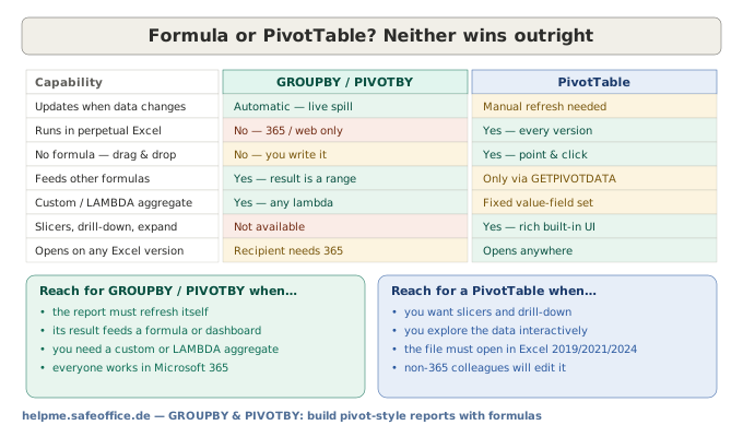
The formula approach is the better choice when the report must be kept in a certain state, when its result must be used to feed another formula, dashboard figure or chart source, or when the report cannot be expressed as a PivotTable but a LAMBDA can. As the formula is text in a cell, it also lends itself well to version control and reviewed, audited workbooks, which is important in regulated or financial settings.
A PivotTable is the better choice when you need to explore data rather than just report on it. You can add a slicer, drill into a figure, expand and collapse groups or restructure the layout by dragging. It is also the answer whenever the file must open on a perpetual licence and works with millions of rows through the Data Model in a way that worksheet formulas do not. When a set of data becomes too big for the grid, using Power Pivot instead of a longer formula is the best next step. See the guide 'Power Pivot and the data model: a beginner's guide' for more information.(/index.php?page=public/en/excel-power-pivot-data-model-beginner-guide).
A useful rule of thumb is that if the output is a deliverable that must stay current independently, use a formula, and if the task involves interactive analysis, use a PivotTable. Many real workbooks use both: a PivotBy feeding a live dashboard and a PivotTable alongside it for ad hoc questions.
Part 7: Availability and the perpetual-licence fallback
GROUPBY and PIVOTBY reached general availability in the Microsoft 365 Current Channel on both Windows and Mac, as well as in Excel for the web, in late 2024. These features are not included in any perpetual licence, including Excel 2016, 2019, 2021 and the perpetual Excel 2024 licence. Workbooks that use these features will open in these versions with the error message _xlfn.GROUPBY and #NAME?. This distinction is significant for German SMEs and public bodies, where perpetual licences are still widespread. The wider picture is set out in Excel 365 versus older versions.
For a one-dimensional summary, UNIQUE and SUMIFS together reproduce most of GROUPBY. On Excel 2021, which has dynamic arrays but not GROUPBY:
=UNIQUE(Sales[Region])                              ' in A2 — spills the distinct regions
=SUMIFS(Sales[Amount], Sales[Region], A2#)          ' in B2 — spills the totals alongside
The A2# spill reference keeps the two columns aligned when regions are added or removed. In Excel 2016 or 2019, where there is no spill, list the regions once using Data ▸ Remove Duplicates and aooly a plain SUMIF on each row. The mechanics of criteria-based summing are covered in SUMIFS: conditional sums with multiple criteria.
For a two-dimensional matrix there is no concise formula equivalent with a perpetual licence; a PivotTable is the correct solution. This is one of the cases in Part 6 where the PivotTable is not a fallback option, but simply the right tool for the job.
Part 8: Common failure modes
| Symptom | Likely cause | Fix |
|---|---|---|
#NAME? or _xlfn.GROUPBY |
Opened in a version without the function | Use UNIQUE + SUMIFS, or a PivotTable; see Part 7 |
#SPILL! |
A cell in the intended spill range is occupied | Clear the cells below and to the right of the formula |
#CALC! |
filter_array removed every row, or an argument is a nested array |
Check the filter; keep row_fields and values as simple columns |
| Wrong column sorted | sort_order counts row_fields first, then values |
Recount from the first column of the report, not column A |
| Totals missing or misplaced | total_depth misread |
0 none, 1 grand, 2 grand plus subtotals; negative places them on top |
| A stray extra header row | field_headers mis-detected |
Set field_headers explicitly (3 = headers present and shown) |
| Lengths do not match | row_fields, values and filter_array differ in height |
Base every argument on full columns of the same table |
Summary
The real significance of GROUPBY and PIVOTBY is that they make report-building a formula task rather than an object-building one.
GROUPBYreturns one row per group, whilePIVOTBYreturns a two-way matrix. Both find the groups for you and both spill.- The report recalculates automatically and can feed other formulas, which is a property that PivotTable do not have.
- Sorting (
sort_order), filtering (filter_array) and totals (total_depth) are arguments, not extra layers. PERCENTOFand customLAMBDAaggregations extend beyond the fixed value-field-menue of a PivotTable, whilerelative_tocan convert a whole matrix into percentages of the row, column or grand-total.- Choose the formula if you need the output to stay current or to feed further calculations. Choose a PivotTable if you want to explore the data interactively, if the data set is very large, or if the file must open on a perpetual licence.
- The functions require Microsoft 365 or Excel for the web. With a perpetual licence, use
UNIQUE+SUMIFSfor a list, or a PivotTable for a matrix.
The principle that runs through this series is to prefer the tool that makes the report both correct and self-maintaining, and to be deliberate about when interactivity or compatibility means that a PivotTable is the better answer.
See also: Dynamic arrays with FILTER, SORT, UNIQUE and SEQUENCE for the spill behaviour these functions rely on, SUMIFS: conditional sums with multiple criteria for the perpetual-licence fallback, Why every dataset should be an Excel table for the structured references that keep these reports stable, Power Pivot and the data model: a beginner's guide for when a dataset outgrows worksheet formulas, and Excel 365 versus older versions for the full availability picture.
This article is part of the helpme.safeoffice.de series, which provides practical guides on Excel functions, workbook modeling and data solutions. The series is aimed at businesses that want effective, maintainable tools that everyone can understand.