Power Pivot and the Data Model in Excel: A Beginner's Guide
FAQ — What does this article answer?
Q: What is the data model, and how does it differ from a normal Excel spreadsheet?
A: The data model is an in-memory database that lives inside your Excel file. It can hold multiple related tables, handle hundreds of millions of rows and perform calculations using a language called DAX. This article explains what that means in practical terms.
Q: Is there anything else I need to buy to use Power Pivot?
A: No, Power Pivot is included in Excel 365, Excel 2021 and Excel 2019. It is hidden by default, but you can enable it as a COM add-in. This article shows you exactly how to do this.
Q: Why would I use the Data Model instead of VLOOKUP to join two tables?
A: VLOOKUP is a formula that runs once per cell. In a table with 500,000 rows, for example, you could end up with 500,000 slow lookups. In contrast, a relationship in the Data Model is a permanent link — Excel resolves it instantly, regardless of scale, so you never need to write a lookup formula again.
Q: What is DAX and do I need to learn a programming language?
A: DAX (Data Analysis Expressions) is a formula language designed for the Data Model. Its simplest formulas, such as SUM, AVERAGE and COUNTROWS, look almost identical to those in Excel. This article starts with these and explains the one new concept that sets DAX apart: filter context.
Q: What is the difference between a measure and a calculated column?
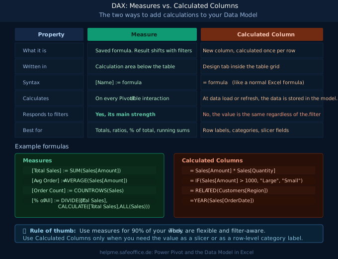
A: A measure is recalculated every time a filter is applied, making it the right choice for totals, ratios and percentages. A calculated column adds a new column to the table with a fixed value per row; use this for labels and categories. Both are covered in this article.
What Power Pivot actually is
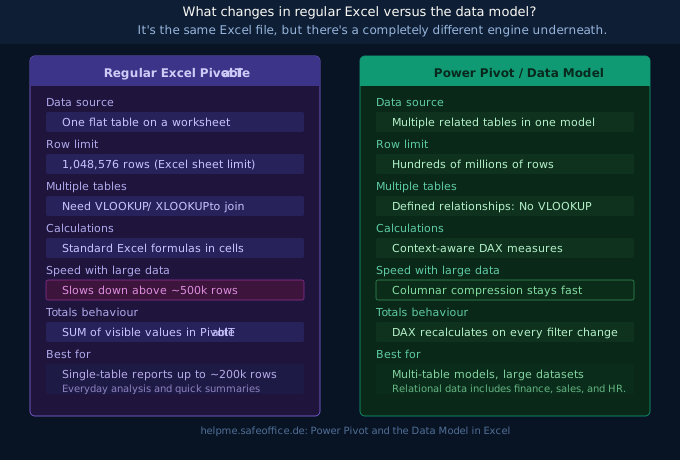
Open a regular Excel PivotTable and you will see that it is just one flat table on a worksheet. However, the Power Pivot engine — also known as the Data Model — replaces this with a far more capable compressed, in-memory column store. This can hold multiple related tables, process millions of rows without slowing down and perform calculations using a formula language designed specifically for analytical work.
The Data Model lives inside your .xlsx file. There is no need for an external server, installation beyond enabling the add-in or a separate tool. It's Excel, but with a much more powerful engine underneath!
Enabling Power Pivot
Power Pivot is disabled by default. Once enabled, it stays on.
- Go to File → Options → Add-ins
- At the bottom, change the Manage dropdown to COM Add-ins and click Go
- Check Microsoft Power Pivot for Excel
- Click OK
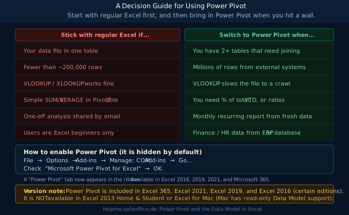
A Power Pivot tab will now appear in your ribbon. This feature is available in Excel 365, Excel 2021 and Excel 2019. It is not available in Excel for Mac, which can read data models but not author them.
Knowing when to use it and when not to is key.
Power Pivot is not a replacement for standard Excel; it's a step up when standard Excel reaches its limits. Before we go any further, it's important to be clear about what that limit is.
Use regular Excel when your data fits in one table, your row count is under 200,000 and a standard PivotTable with SUM or AVERAGE functions provides the required results. This covers the majority of everyday analysis.
Switch to Power Pivot when:
- you need to join two or more tables without VLOOKUP
- your data has hundreds of thousands of rows and the file is slow
- you need calculations such as percentage of total, year-to-date or rolling averages.
- You run the same report every month using freshly exported data.
The data model comprises multiple tables and one model.
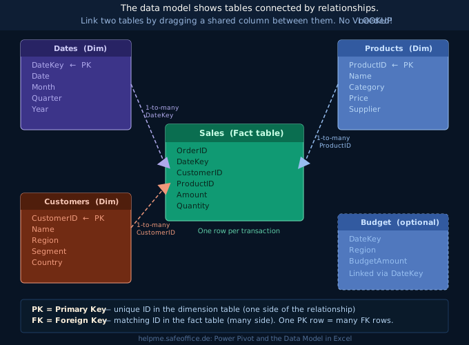
The most important concept in Power Pivot is the relationship. Rather than copying data from one table to another using VLOOKUP, you inform Excel of the connection between the tables. From that point on, Excel automatically resolves the connection at any scale and for every PivotTable interaction.
Fact tables and dimension tables
In any well-structured data model, there are two types of table.
Fact tables hold transactional data, with one row for each sale, order or event. They tend to be wide with many rows. A 'Sales' table containing columns such as 'OrderID', 'DateKey', 'CustomerID', 'ProductID', 'Amount' and 'Quantity' is a typical fact table.
Dimension tables hold descriptive data, such as one row per customer, one row per product and one row per date. They are smaller and provide the labels and categories by which you can analyse your facts. A 'Customers' table with one row per customer (CustomerID, Name, Region, Segment) is a typical dimension table.
The column that acts as the connection between the two tables is called the primary key (PK) in the dimension table and the foreign key (FK) in the fact table. A dimension table contains one row for each key value. The fact table has multiple rows per key value. This is a one-to-many relationship.
Creating relationships
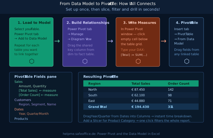
- Load your tables into the data model. Click inside each Excel table, go to the Power Pivot tab and click Add to Data Model. Repeat for each table.
- In the Power Pivot window, click Diagram View on the Home tab. Your tables will appear as boxes.
- Drag the primary key column from the dimension table onto the matching foreign key column in the fact table. A line will appear between them; this is the relationship.
From this point onwards, any PivotTable created using the Data Model can combine fields from all linked tables without the need for VLOOKUP.
DAX is the formula language of the data model.
DAX stands for 'Data Analysis Expressions'. It is the language used to create calculations within the Data Model. Many DAX functions have the same names as their Excel counterparts, such as SUM, AVERAGE, MIN, MAX and IF, and work in a similar way. The key difference is that DAX formulas always operate on entire columns or tables rather than individual cells.
Your first measures
A measure is a saved calculation that exists in the data model. Once you have written it in the Power Pivot window, it becomes available in every PivotTable that uses the model. The syntax uses := instead of =:
[Total Sales] := SUM(Sales[Amount])
[Order Count] := COUNTROWS(Sales)
[Average Order] := AVERAGE(Sales[Amount])
To write a measure, click an empty cell in the grey Calculation Area below a table in the Power Pivot window and type your formula in the formula bar above.
The one new idea: filter context.
What sets DAX apart from Excel formulas is filter context: the concept whereby a measure is recalculated based on the filters currently applied to the PivotTable.
Place [Total Sales] in a PivotTable and drag Region into the rows. The measure will automatically show the total for each region, not because a different formula has been written for each row, but because the PivotTable applies a filter for each region and the measure responds to this. Add a Year slicer and the measure will respond to that too. Every combination of filters produces the correct result from a single measure.
This is why you should write most of your calculations as measures rather than hard-coded formulas.
CALCULATE is the most important DAX function
CALCULATE runs a measure inside a modified filter context. In other words, it allows you to modify the data that the formula sees before it calculates.
[North Sales] := CALCULATE([Total Sales], Customers[Region] = "North")This always shows the total for North, regardless of the region filter applied in the PivotTable, which is useful for comparison columns.
[% of Total] := DIVIDE([Total Sales], CALCULATE([Total Sales], ALL(Sales)))ALL(Sales) removes all filters from the Sales table, providing the grand total. DIVIDE produces the percentage for the current filter context. A single formula automatically delivers the correct percentage for every row in the PivotTable.
Building the PivotTable from the Data Model
Once you have added tables, relationships and measures to your model, creating the report is easy:
- Go to Insert → PivotTable
- Select From Data Model (not From Table/Range)
- In the PivotTable Fields pane you will now see all your tables listed, rather than just one flat list of columns.
Drag fields from any linked table into the PivotTable. As the relationships have already been defined, Excel knows how to combine them. Drag Region from Customers into Rows and drag [Total Sales] from Sales into Values. The PivotTable will immediately show total sales per region, calculated correctly across the relationship.
Add a Slicer for any dimension, such as Year, Product Category or Sales Segment, and every measure will update simultaneously when you click. Add multiple PivotTables connected to the same model and they will all respond to the same slicers.
Practical tips for beginners
Name your tables before loading them. Select your data, press Ctrl+T, then go to Table Design and give the table a meaningful name, such as Sales or Customers. These names will appear in DAX formulas and in the Fields pane, so clear names will make everything more readable.
Start with three measures: before exploring advanced DAX, familiarise yourself with SUM, COUNTROWS and DIVIDE. Ninety percent of reporting questions can be answered with these three measures.
Use DIVIDE instead of dividing directly, as =A/B will crash if B is zero. =DIVIDE(A,B) returns a blank, which is much cleaner in a PivotTable.
Keep dimension tables small and clean. Your 'Dates' table should contain one row for each calendar date and include useful columns such as Month, Quarter, Year and Weekday Name. You can generate this using the SEQUENCE function in a spreadsheet and then load it into the model.
Do not mix fact data and dimension data in one table: if your sales table contains the customer's name and region repeated on every row, this is redundant data. Split it out into a proper Customers dimension; the relationship will handle the connection.
Summary
| Concept | What it means |
|---|---|
| Data Model | An in-memory database inside your Excel file — multiple tables, millions of rows |
| Relationship | A permanent link between tables via a shared key column — replaces VLOOKUP |
| Fact table | Many rows of transactional data (Sales, Orders, Events) |
| Dimension table | One row per entity — provides labels and categories (Customers, Products, Dates) |
| DAX Measure | A filter-aware calculation — recalculates on every PivotTable interaction |
| DAX Calculated Column | A row-level value stored in the model — use for labels and slicer fields |
| CALCULATE | Runs a measure with a modified filter — the most powerful DAX function |
| Filter context | The set of filters the PivotTable applies when a measure calculates |
Power Pivot is a worthwhile investment. Once you grasp the concept of relationships and measures, problems that previously required complex VLOOKUP formulas, helper columns or heavy calculations can be solved with just a few lines of DAX and an updatable PivotTable.