Note: In Article 2, you will find the link to download the workbook (EXE file).

Part 04: Closing the Loop — CATEGORIE_STIMATE_VS_EFFETTIVE and REGISTRO_ENTRATE_&_USCITE

Overview

The first two articles explained how the workbook creates a cost baseline and monitors actual expenditure. This final article examines where these two processes converge. CATEGORIE_STIMATE_VS_EFFETTIVE (Budget Categories: Estimate vs. Actual) is the variance report, providing a clear summary of how each category is performing against the budget. REGISTRO_ENTRATE_&_USCITE (Income and Expenditure Register) is the raw transaction ledger that feeds everything upstream. Together, these two reports complete the data pipeline: transactions enter through the ledger, flow through the actual cost sheet and appear as variance figures in the comparison report.

Sheet 3: CATEGORIE_STIMATE_VS_EFFETTIVE

Purpose

This sheet adresses the fundamental question of project control: which budget categories are on track, and which are not? It provides a three-column comparison of estimated budget, actual cost, and variance for every category, with column totals for each column at the top.

The sheet is intentionally simple. There is no complex time phasing here; this work has already been done in Sheets 1 and 2. This Sheet's job is ti summaries those time-phased arrays into a single line per category, making any divergences immediately visible.

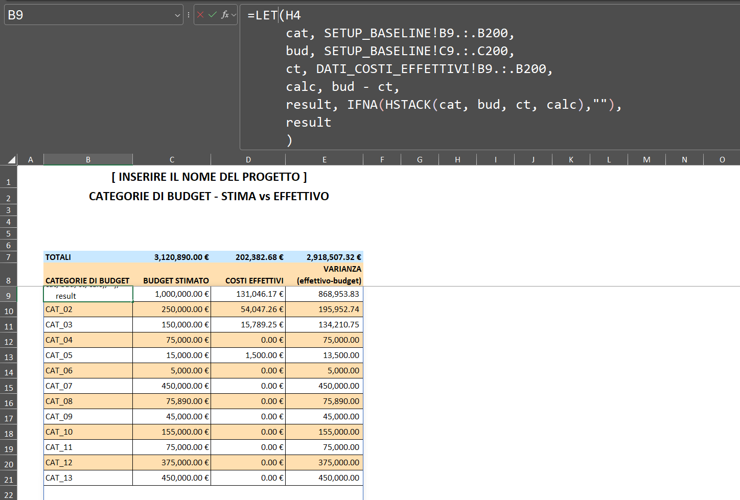
The LET Formula in B9

The category column (B9) is populated by a single LET formula that retrieves category data and creates the comparison table.

=LET(
   cat,  _TRO_ALL(SETUP_BASELINE!B9:B200),
   bud,  _TRO_ALL(SETUP_BASELINE!C9:C200),
   ct,   _TRO_ALL(DATI_COSTI_EFFETTIVI!B9:B200),
   calc, IFNA(HSTACK(cat, bud, ct), ""),
   calc
)

Three arrays are defined:

• cat — the category names from SETUP_BASELINE
• bud — the estimated budget from SETUP_BASELINE
• ct — the actual total costs from the B column of Sheet 2 (which are themselves produced by the SUMIF formula described in Article 2)

HSTACK it assembles these three arrays side by side to create a single spilled output covering columns B, C, and D. IFNA(..., "") suppresses rows where any value is an error, typically empty rows at the bottom of the 200-row range.

The Variance Column (E9)

Column E is simply:

=SUM(C9:C200)  [row 7 total]

The variance for each row is the calculated difference between the actual spend (column D) and the budget (column C). In the current data, all variances are positive because the actual spend is lower than the budget — the project is still in progress and costs are accumulating.

Column Totals (Row 7)

C7: =SUM(C9:C200)
D7: =SUM(D9:D200)
E7: =SUM(E9:E200)

These plain SUM formulas work correctly, even though C9:C200, D9:D200, and E9:E200 are populated by the spillover from B9. Excel recognises spilled ranges within SUM — the totals update automatically whenever new categories are added or budgets change in SETUP_BASELINE.

Sheet 4: REGISTRO_ENTRATE_&_USCITE

Purpose

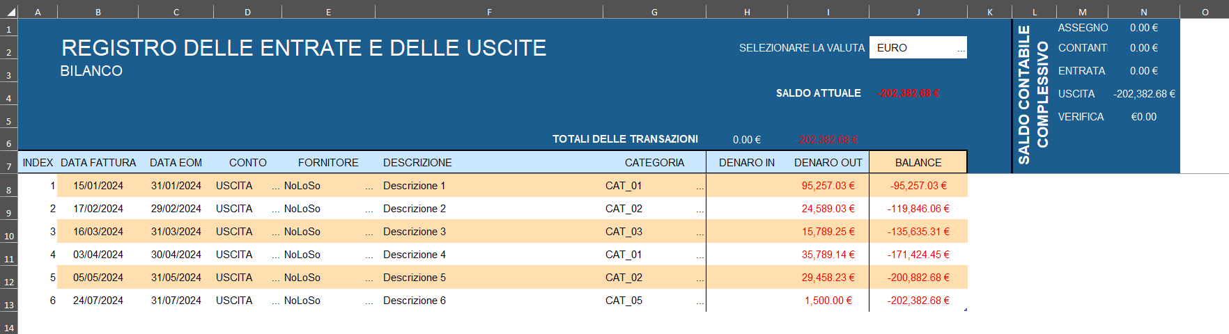
The ledger is the single source of truth for all financial activity. Every payment made — every invoice received, every income item — is recorded here as a row in the structured table tbl_Registro_UE. This table drives the actual cost totals in Sheet 2 and, by extension, the variance figures in Sheet 3.

The sheet also functions as a standalone financial register, with its own balance tracking and per-account summary panel.

The Structured Table: tbl_Registro_UE

The transaction data is stored as a formal Excel table rather than a plain range. This has several architectural implications:

1. Structured references — formulas elsewhere in the workbook can refer to columns by name (tbl_Registro_UE[CATEGORIA], tbl_Registro_UE[DENARO OUT]) rather than by address. This makes formulas self-documenting and resilient to column reordering.
2. Automatic expansion — when a new row is added to the table, all dependent formulas (particularly the SUMIFS in Sheet 2) automatically include the new data without any manual range adjustment.
3. Consistent column types — the table enforces column-level data types, reducing the risk of mixed text/number entries that would break SUMIFS matching.

The table columns are: INDEX, DATA FATTURA (invoice date), DATA EOM (end-of-month date), CONTO (account), FORNITORE (supplier), DESCRIZIONE (description), CATEGORIA (category), DENARO IN (money in), DENARO OUT (money out), BALANCE.

The Auto-Index Formula (Column A)

Cell A8 contains a dynamic array formula that automatically numbers all rows:

=SEQUENCE(COUNT(--tbl_Registro_UE[DATA EOM]),, 1, 1)

COUNT(--tbl_Registro_UE[DATA EOM]) counts the number of non-blank rows in the DATA EOM column. The double-negative (--) which can be read more about here coerces date values to numbers so that the COUNT function recognises them. SEQUENCE(n,, 1, 1) produces a vertical array from 1 to n, and the result always matches the current number of data rows. No manual renumbering is needed when rows are added.

The DATA EOM Column (Column C)

Every transaction has its invoice date (DATA FATTURA) normalised to the last day of its calendar month:

=IF($B8="", "", EOMONTH(B8, 0))

The EOMONTH(date, 0) function returns the last day of the month containing the specified date. The IF guard returns a blank value when no invoice date is present. This normalisation bridges the gap between the raw ledger and the distribution matrix in Sheet 2. By aligning all transactions to their end-of-month date, the SUMIFS function in Sheet 2 can match them to the correct monthly column using a simple equality test.

The Running Balance Column (Column J)

The BALANCE column tracks cumulative net position after each transaction. The formula is:

=SUBTOTAL(9, tbl_Registro_UE[[#Headers],[DENARO IN]]:tbl_Registro_UE[[#This Row],[DENARO IN]])
-SUBTOTAL(9, tbl_Registro_UE[[#Headers],[DENARO OUT]]:tbl_Registro_UE[[#This Row],[DENARO OUT]])

This uses the SUBTOTAL function with the (sum) function code 9 in an expanding range pattern. The range starts at the column header ([#Headers]) and ends at the current row ([#This Row]). As the start point is fixed at the header and the end point moves with each row, the sum expands row by row, producing a cumulative total.

The key advantage of using SUBTOTAL rather than SUM here is that SUBTOTAL is filter-aware: if the table is filtered to show only certain categories or date ranges, SUBTOTAL recalculates the balance based only on visible rows. A simple SUM would ignore the filter.

The net balance formula in the header area (cell J4) uses a simpler version:

=H6 - I6

Where H6 and I6 are the transaction totals for DENARO IN and DENARO OUT respectively, themselves calculated as:

H6: =SUBTOTAL(9, tbl_Registro_UE[[#All],[DENARO IN]])
I6: =SUBTOTAL(9, tbl_Registro_UE[[#All],[DENARO OUT]])

The 'Per-Account Balance Summary' Panel

A compact panel displaying the net balance for each registered account is located in the top-right of the sheet (columns M–N). Account names are pulled from SETUP_REGISTRO.

M1: =IF(SETUP_REGISTRO!B2="", "", SETUP_REGISTRO!B2)
M2: =IF(SETUP_REGISTRO!B3="", "", SETUP_REGISTRO!B3)
...

Each account's balance is calculated by:

N1: =IF(M1="", "",
     SUMIFS(tbl_Registro_UE[[#All],[DENARO IN]],  tbl_Registro_UE[[#All],[CONTO]], M1)
   - SUMIFS(tbl_Registro_UE[[#All],[DENARO OUT]], tbl_Registro_UE[[#All],[CONTO]], M1)
)

Here, the SUMIFS function filters by account name in the CONTO column, summing all inflows and outflows for each account separately before subtracting them to determine the net position. The IF(M1="", "", ...) wrapper ensures that blank account slots display as empty rather than showing a zero.

The Full Data Pipeline

Now that all four sheets have been described, it is useful to visualise how data flows through the workbook from entry to reporting.

SETUP_BASELINE
  │  Project parameters, category list, working day counts
  │
  ├──► AUTO_PROSPETTO_COSTI  (Sheet 1)
  │      MAKEARRAY × NETWORKDAYS.INTL → time-phased cost baseline
  │
  └──► DATI_COSTI_EFFETTIVI  (Sheet 2)
         LET/HSTACK pulls category list
         SUMIFS (2D) against tbl_Registro_UE → time-phased actuals
              │
              ▼
REGISTRO_ENTRATE_&_USCITE  (Sheet 4)
  tbl_Registro_UE (structured table)
  EOMONTH normalisation → DATA EOM
  SUBTOTAL running balance
              │
              ▼
CATEGORIE_STIMATE_VS_EFFETTIVE  (Sheet 3)
  LET/HSTACK: cat + bud (Sheet 1) vs ct (Sheet 2) → variance report

Every update to the ledger is propagated upwards automatically. For example, adding a new invoice in Sheet 4 instantly updates the actual cost totals in Sheet 2, which are then immediately reflected in the variance figures in Sheet 3 — there is no need for manual refreshing or copying and pasting.

Key Takeaways

Sheet 3:

• A LET/HSTACK formula combines the three-column comparison from SETUP_BASELINE and Sheet 2 into a single spill — the entire table is driven by one formula.
• Column totals use simple formula SUM against the spilled ranges and update automatically.
• Variance is budget minus actuals, expressed as a positive number when under budget.

Sheet 4:

• The structured table tbl_Registro_UE uses named columns throughout, which makes all dependent formulas readable and robust to structural changes.
• The critical link that enables two-dimensional SUMIFS matching in Sheet 2 is the EOMONTH normalisation in the DATA EOM column.
• The running balance uses the SUBTOTAL function in an expanding structured reference. This gives a cumulative net position that respects table filters.
• The per-account balances displayed in the summary panel are calculated using the SUMIFS function, filtered by the CONTO column and driven by the account names stored in the SETUP_REGISTRO table.

Visualisations (this article)

Diagram 1 — The full workbook data pipeline. End-to-end flow from SETUP_BASELINE through Sheets 1, 2, and 4, converging at the variance report in Sheet 3.

Diagram 2 — SUBTOTAL expanding range: how the running balance is built. Row-by-row illustration of how the structured reference [#Headers]:[#This Row] expands with each new transaction, and why SUBTOTAL is preferred over SUM for filter-awareness.

See also:
Before the formulas, the architecture (Cost Baseline Expenditure Schedule Part 01),
How a single formula builds an entire time-phased cost baseline. (Cost Baseline Expenditure Schedule Part 02) and
Data flows of a ledger into a time-phased actual cost matrix. (Cost Baseline Expenditure Schedule Part 03)