FAQ — What Does This Article Answer?

What is MAKEARRAY, and why would I use it instead of copying a formula across cells?

A: MAKEARRAY is an Excel 365 function that creates a matrix of values from a single formula. Rather than placing a formula in each cell and copying it across rows and columns, MAKEARRAY calculates all the values in a single operation. This means that the logic exists in one place only. If you need to change it, you only need to change one formula and the entire matrix will update. There is nothing to copy, nothing to break and nothing to overlook.

What does LET actually do within a formula?

A: It assigns names to intermediate values or calculations, allowing them to be reused in the same formula without the need for repeated calculations. This process is similar to defining variables in a programming language. Rather than writing the same complex expression three times, you write it once, give it a name and then refer to that name. This makes formulas shorter and faster, and readable by anyone who opens them — not just the person who wrote them.

Why does the formula return 'NA' instead of '0' for months where a category has no spending?

A: The formula returns NA rather than zero on purpose, using the expression IF(monthlyDays = 0, NA(), dailyRate * monthlyDays). This is an intentional design choice. 'Zero' means 'this category has zero planned spending this month'. NA means 'this category does not exist at all this month.' Most chart types skip NA cells entirely, while zero cells are plotted as a data point at zero. Using NA produces cleaner, more accurate charts.

How does the formula know which public holidays to exclude from working day calculations?

A: The named range _DataFestivita refers to a dedicated sheet called feste_italia_sardegna containing 52 public holiday dates for the years 2024, 2025 and 2026, including Italian national holidays and the Sardinian regional holiday 'Sa die de sa Sardigna' on 28 April. This range is passed directly into NETWORKDAYS.INTL as the holidays parameter, meaning that every working day calculation in the entire matrix automatically excludes these dates, eliminating the need for manual adjustment.

What happens if a category's dates are missing or incorrect?

A: Every date calculation in the formula is wrapped in an IFERROR function with a safe fallback value. If a task start date is missing, IFERROR(taskStart, DATE(2100,1,1)) substitutes a date far in the future. This ensures the MAX calculation for period overlap will never produce a negative result. Similarly, if a task end date is missing, the formula IFERROR(taskEnd, DATE(1900,1,1)) substitutes the earliest possible Excel date, to ensure that the MIN calculation collapses the period to nothing. The outer IFERROR then catches anything that still produces an error and returns an empty string instead.

Inside the formula, there is a way to build a cost baseline from a single cell. This is done using MAKEARRAY, LET and LAMBDA.

This workbook contains a formula that sits in a single cell and produces 156 values simultaneously.

This formula calculates the monthly cost distribution for 13 budget categories across 12 months. It also accounts for Italian national and Sardinian regional public holidays, handles categories that start or end mid-month correctly and protects against missing dates and division by zero. Furthermore, it returns 'NA' rather than zero for months where a category has no planned spending.

It does all this without a single visible error. And it does all this from one cell.

This article uses a formula explorer to break down the formula, showing the intermediate value at each step and making visible what would otherwise require in-depth Excel expertise to understand.

The aim is not to encourage you to write formulas like this. Rather, the aim is to demonstrate what is possible, explain why it was designed in this way, and highlight the factors that contribute to its maintainability rather than its fragility.

The full formula:

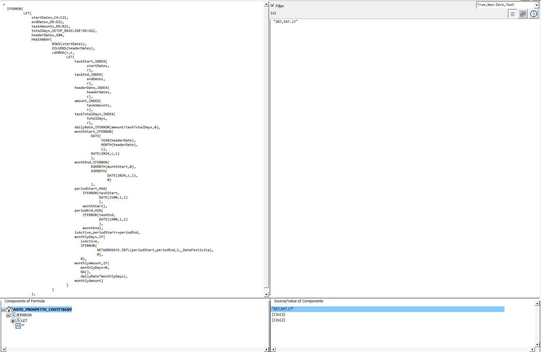
This is the complete formula from cell AUTO_PROSPETTO_COSTI!$G$9, exactly as it appears in the formula bar:

=IFERROR(LET(
    startDates, C9:C21,
    endDates, D9:D21,
    taskAmounts, B9:B21,
    totalDays, SETUP_BASELINE!G9:G21,
    headerDates, G8#,
    MAKEARRAY(
        ROWS(startDates),
        COLUMNS(headerDates),
        LAMBDA(r,c,
            LET(
                taskStart, INDEX(startDates, r),
                taskEnd, INDEX(endDates, r),
                headerDate, INDEX(headerDates, c),
                amount, INDEX(taskAmounts, r),
                taskTotalDays, INDEX(totalDays, r),
                dailyRate, IFERROR(amount / taskTotalDays, 0),
                monthStart, IFERROR(DATE(YEAR(headerDate), MONTH(headerDate), 1), DATE(2024, c, 1)),
                monthEnd, IFERROR(EOMONTH(monthStart, 0), EOMONTH(DATE(2024, c, 1), 0)),
                periodStart, MAX(IFERROR(taskStart, DATE(2100, 1, 1)), monthStart),
                periodEnd, MIN(IFERROR(taskEnd, DATE(1900, 1, 1)), monthEnd),
                isActive, periodStart <= periodEnd,
                monthlyDays, IF(isActive,
                    IFERROR(NETWORKDAYS.INTL(periodStart, periodEnd, 1, _DataFestivita), 0),
                    0
                ),
                monthlyAmount, IF(monthlyDays = 0, NA(), dailyRate * monthlyDays),
                monthlyAmount
            )
        )
    )
),"")

At first, this may seem like a wall of text. However, by the end of the article, every line will make sense.

A structural overview of how the layers nest

The formula comprises four distinct layers, each with a specific function. Understanding the function of each layer independently makes the whole much easier to read.

Layer 1 - IFERROR: The safety net. If any part of the formula produces an error for any reason, IFERROR detects it and returns an empty string instead. The user never sees an error. This outer wrapper makes the workbook presentable, even if the data is incomplete.

Layer 2 - Outer LET: The preparation stage. Before any calculations are performed, LET collects all the data that the formula requires and gives each piece a clear name. Five named variables are defined here: startDates, endDates, taskAmounts, totalDays and headerDates. Everything that follows uses these names rather than raw cell references.

Layer 3 — MAKEARRAY: The Matrix Builder. MAKEARRAY is instructed to create a grid containing 13 rows and 12 columns. For each position in the grid, the LAMBDA function is called with the row number r and the column number c.

Layer 4 — LAMBDA with inner LET: The calculation engine. For each row-column combination, the inner LET statement defines additional named variables and performs the monthly cost calculation.

The ins and outs of Layer 2 — the names and the reasons why they matter

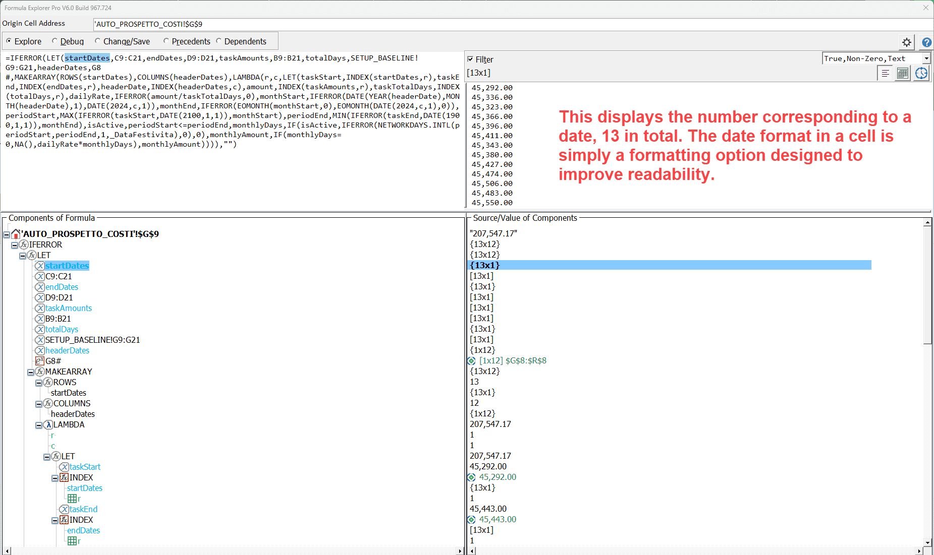
When formula explorer highlights 'startDates' in the component tree, the value is displayed in the right panel: a column of 13 dates in Excel serial number format. These are the start dates of all 13 budget categories and are read directly from cells C9:C21 in the same spreadsheet.

The same pattern applies to all five named variables.

The G8# reference for headerDates deserves special attention. The # symbol means 'wherever this formula spills to'; it is a dynamic spill reference. If the project duration changes and additional month columns are added, headerDates automatically expands to include them. MAKEARRAY then builds a wider matrix without requiring any manual updating of the formula.

This is what a single source of truth means in practice. Change the project dates in SETUP_BASELINE and the formula will adapt automatically.

Layer 3 in detail: how MAKEARRAY is built.

The MAKEARRAY function receives three arguments: the number of rows, the number of columns, and a LAMBDA function to be called for each position.

ROWS(startDates) evaluates to 13, as there are 13 budget categories. COLUMNS(headerDates) evaluates to 12, as there are 12 columns for the months.

MAKEARRAY then calls LAMBDA(r, c, ...) 156 times, once for every combination of row and column. On the first call, r = 1 and c = 1 (category 1, month 1). On the final call, r = 13 and c = 12 (category 13, month 12).

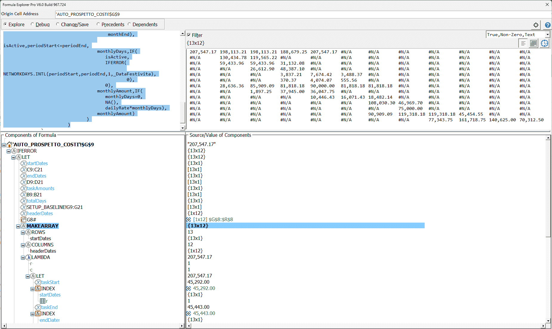
The output panel in the explorer shows the complete 13×12 matrix. Most cells contain a monetary value. Many contain #N/A — these are the months for which that category has no planned spending. These #N/A values are intentional, as explained in the FAQ above.

Layer 4 in detail: the calculation engine for each cell.

The inner LET function defines 12 named variables for each row-column position. Reading them in order reveals the full calculation process:

taskStart and taskEnd are retrieved from startDates and endDates, respectively, using INDEX with the current row number, r. For row 1, these are the start and end dates of CAT_01.

headerDate is retrieved from headerDates using INDEX with the current column number c. For column 1, this is the first month header: 1 February 2024 in this workbook.

amount and taskTotalDays: the budget amount and total working days for this category, both retrieved by row.

`dailyRate:IFERROR(amount / taskTotalDays, 0). The budget divided by the total number of working days gives the cost per working day. The IFERROR function protects against division by zero iftaskTotalDays` is zero.

monthStart and monthEnd: the first and last days of the current month. monthStart is calculated as DATE(YEAR(headerDate), MONTH(headerDate), 1), i.e. the first day of the month. monthEnd is EOMONTH(monthStart, 0), which is the last day of the same month. Both are wrapped in an IFERROR function with a fallback date in case the header date is missing.

periodStart and periodEnd: the overlap calculation

This is the part of the formula that is the most technically interesting.

periodStart, MAX(IFERROR(taskStart, DATE(2100,1,1)), monthStart)
periodEnd,   MIN(IFERROR(taskEnd,   DATE(1900,1,1)), monthEnd)

periodStart is the later of the task's start date and the start date of the month. For example, if the task starts on 15 February but the month starts on 1 February, the period start date is 15 February, as the task was not active for the first two weeks of the month.

periodEnd is the earlier of the task's end date and the end of the month. If the task ends on 10 March, but the end of the month is on 31 March, then the period end is 10 March, as the task was not active for the last three weeks of the month.

The IFERROR fallbacks are deliberate: if taskStart is missing, a date far in the future (year 2100) is substituted so that periodStart is later than periodEnd, making isActive FALSE. If taskEnd is missing, the earliest Excel date (year 1900) is substituted so that periodEnd will be earlier than periodStart, again making isActive FALSE.

isActive

isActive, periodStart <= periodEnd

This single expression determines whether this category overlaps with this month. If the start of the period (periodStart) is on or before the end of the period (periodEnd), the category was active at some point during the month. The result is either TRUE (1) or FALSE (0).

As shown in the screenshot above, when isActive is set to FALSE, the working day calculation is skipped entirely and monthlyDays is set to zero. This boolean gate controls the entire cost calculation.

monthlyDays

monthlyDays, IF(isActive,
    IFERROR(NETWORKDAYS.INTL(periodStart, periodEnd, 1, _DataFestivita), 0),
    0)

When isActive is true, NETWORKDAYS.INTL counts the working days between periodStart and periodEnd, excluding weekends and the 52 Italian and Sardinian public holidays stored in _DataFestivita. The result is the number of working days that this category was active during the current month.

When isActive is False, the result is zero immediately and NETWORKDAYS.INTL is never called.

The IFERROR function surrounding the NETWORKDAYS.INTL function catches one specific edge case: when periodStart is slightly after periodEnd due to a rounding or date precision issue, NETWORKDAYS.INTL returns a negative number. IFERROR detects this and returns zero instead.

monthlyAmount — the final result

monthlyAmount, IF(monthlyDays = 0, NA(), dailyRate * monthlyDays)

If monthlyDays is zero, either because the category was inactive or because the overlap period contained no working days (for example, a period that falls entirely on weekends and public holidays), the result is NA. Otherwise, the result is dailyRate * monthlyDays: the cost per working day multiplied by the number of qualifying working days in the current month.

The last line of the inner LET is simply 'monthly Amount'. This tells LET to return this value. It should be returned as the output for this row-column position.

Why does this architecture matter for maintenance?

A formula this complex could easily become unmanageable. However, it does not, for three specific reasons.

Firstly, there is one formula and one change point: all 156 values in the matrix come from a single formula in G9. If the distribution logic needs to change, for example, if weekend days should be included or a different holiday calendar used, the change only needs to be made in one place. The entire matrix updates.

Named variables and readable logic. Every intermediate value has a descriptive name. isActive, dailyRate, periodStart and monthlyDays are examples of words that a project manager can understand. Compare this to the following formula: =IF(MAX(C9,G$8)<=MIN(D9,EOMONTH(G$8,0)),NETWORKDAYS.INTL(MAX(C9,G$8),MIN(D9,EOMONTH(G$8,0)),1,...)*(B9/SETUP_BASELINE!G9),NA(), which uses the same logic but lacks names. Correct, but unreadable.

Protected edge cases: every point at which an error could occur, such as division by zero, missing dates or negative working day counts, is protected by a specific IFERROR function with a specific fallback. This ensures that the formula behaves correctly rather than producing a visible error.

The formula explorer reveals information that is not present in the formula bar.

The formula bar shows you what the formula says. The formula explorer shows you what the formula does at every step, for every variable and with every intermediate value.

Without the explorer, understanding the formula requires you to mentally simulate the entire calculation chain. With the explorer, however, you can select any variable in the component tree, and the right-hand panel will show its actual value. For example, you can see that _DataFestivita resolves to 52 rows of holiday dates. You can also see that isActive is set to FALSE for a specific cell because periodStart is set to 45,627 and periodEnd is set to 45,322. These two date serial numbers indicate that this category's active period does not overlap with this month's period. You can also see that if IFERROR did not catch it, NETWORKDAYS.INTL would return -213, a negative number that would produce a negative cost if left unchecked.

This illustrates the difference between reading a map and walking the terrain. The formula bar is like a map. You are the explorer.

About this workbook

This article analyses a workbook that is a project cost baseline and expenditure schedule built for construction sector clients operating in Italy. It uses dummy data for demonstration purposes. The companion article covers the complete workbook structure, analysis results and architecture.

Read also: What a workbook analysis really reveals and why not everything that looks wrong actually is

This article is part of the helpme.safeoffice.de series, which provides practical guides on data solutions, workbook modeling and process documentation. The series is aimed at businesses that want effective, long-lasting tools that everyone can understand.