HOME / FORMULAS & FUNCTIONS

Note: In Article 2, you will find the link to download the workbook (EXE file).

Part 03: Recording Reality — `DATI_COSTI_EFFETTIVI`

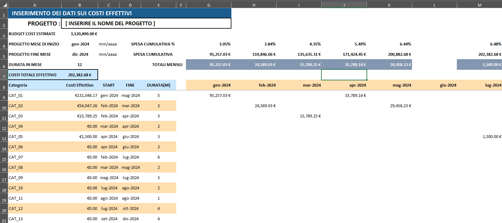
What This Sheet Does

DATI_COSTI_EFFETTIVI — Actual Cost Data Entry — is the live counterpart to the planning sheet covered in Article 1. Where AUTO_PROSPETTO_COSTI describes what was planned, this sheet tracks what was actually spent. Its structure mirrors the baseline sheet almost exactly: the same categories, the same monthly columns, the same summary rows. But the source of the numbers is fundamentally different. Instead of distributing estimated budgets by working-day proration, this sheet reads directly from the transaction ledger (REGISTRO_ENTRATE_&_USCITE) and aggregates real invoice data into the same time-phased format.

This parallel structure is what makes the workbook powerful: because both sheets use the same layout, differences between planned and actual spend become immediately comparable, and the variance analysis in Sheet 3 requires no additional transformation.

Structure at a Glance

The sheet is divided into the same two zones as Sheet 1:

Columns A–E (rows 9 onwards): Category labels, total actual costs, start dates, end dates, and duration — pulled automatically from SETUP_BASELINE and from the ledger.
Columns G onwards: The actual cost matrix. Each column is a calendar month; each cell shows the real amount spent on that category in that month, sourced from invoices in the ledger.

Rows 4–7 carry the same summary structure as Sheet 1: actual monthly totals, cumulative actuals, and cumulative actuals as a percentage of the total budget estimate.

Illustrating the data

The Month Header Row: A Different Approach

In Sheet 1, the month header in row 8 generates dates based on the project's planned start and end. In Sheet 2, the approach is slightly different. Cell G8 is anchored to the actual start date:

=EOMONTH(ACTUALSTARTDATE, 0)

This returns the last day of the month containing ACTUALSTARTDATE. Cell H8 then dynamically extends the series:

=EOMONTH(
   EDATE(G8, SEQUENCE(, MONTH(ACTUALENDDATE) - MONTH(ACTUALSTARTDATE))),
   0
)

Where Sheet 1 produces the first day of each month, Sheet 2 produces the last day (end-of-month dates). This is deliberate: the ledger sheet (REGISTRO_ENTRATE_&_USCITE) stores a calculated DATA EOM column (end-of-month date) for each transaction. Using end-of-month dates in both places means the SUMIFS lookup in the distribution formula can match exactly on this field, avoiding any ambiguity caused by transactions recorded on different days within the same month.

Named ranges used:

ACTUALSTARTDATE → DATI_COSTI_EFFETTIVI!$B$4
ACTUALENDDATE → DATI_COSTI_EFFETTIVI!$B$5

The Input Rows: A `LET` That Aggregates from the Ledger

Cell A9 contains a LET formula that populates the entire input table. It differs from its Sheet 1 counterpart in one critical way: the cost column (ct) is not read from SETUP_BASELINE but calculated live by summing all matching transactions from the ledger table:

=LET(
   cat,    SETUP_BASELINE!B9:B200,
   ct,     SUMIF(tbl_Registro_UE[CATEGORIA], cat, tbl_Registro_UE[DENARO OUT]),
   inizio, SETUP_BASELINE!D9:D200,
   fine,   SETUP_BASELINE!E9:E200,
   durata, SETUP_BASELINE!F9:F200,
   result, IFNA(HSTACK(cat, ct, inizio, fine, durata), ""),
   result
)

The key line is:

ct, SUMIF(tbl_Registro_UE[CATEGORIA], cat, tbl_Registro_UE[DENARO OUT])

SUMIF here operates in array mode because cat is an array (the full column B9:B200 from SETUP_BASELINE). Excel evaluates SUMIF once for each value in cat, returning an array of totals — one per category. This means ct holds the sum of all outgoing payments tagged with each category name, sourced directly from the structured table tbl_Registro_UE.

HSTACK then assembles category names, actual totals, dates, and duration into a single spilled output. The formula in B7 separately confirms the grand total:

=SUM(B9:B200)

Because B9:B200 is populated by the spill from A9, this sum dynamically reflects whatever the LET formula produces.

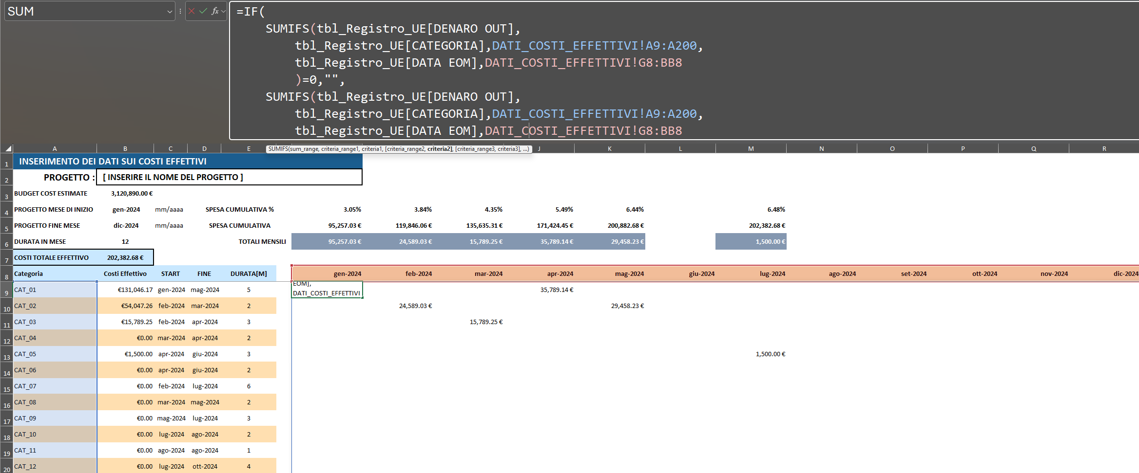
The Core Distribution Formula: `SUMIFS` Across Two Dimensions

The cell G9 formula in Sheet 2 is elegant in its simplicity compared to the working-day calculation of Sheet 1. Since actual costs are discrete invoice events with a specific date, there is no need to prorate by day — the question is simply: which invoices belong to this category and fall in this month?

=IF(
   SUMIFS(
      tbl_Registro_UE[DENARO OUT],
      tbl_Registro_UE[CATEGORIA],    DATI_COSTI_EFFETTIVI!A9:A200,
      tbl_Registro_UE[DATA EOM],     DATI_COSTI_EFFETTIVI!G8:BB8
   ) = 0,
   "",
   SUMIFS(
      tbl_Registro_UE[DENARO OUT],
      tbl_Registro_UE[CATEGORIA],    DATI_COSTI_EFFETTIVI!A9:A200,
      tbl_Registro_UE[DATA EOM],     DATI_COSTI_EFFETTIVI!G8:BB8
   )
)

This is a two-dimensional SUMIFS that exploits Excel's dynamic array behaviour. Here is why it works:

A9:A200 is a vertical array of category names (one per row).
G8:BB8 is a horizontal array of end-of-month dates (one per column).

When SUMIFS receives arrays for both criteria ranges simultaneously, Excel broadcasts the calculation across both dimensions, returning a matrix — one row per category, one column per month — in a single formula. Each cell in the matrix is the sum of all DENARO OUT values in the ledger where the category matches and the DATA EOM date matches.

The IF(...=0, "", ...) wrapper suppresses zeros, keeping empty months visually blank rather than displaying 0.

Formula bar visible, alongside the surrounding data showing

Summary Rows: Mirroring Sheet 1

The three summary rows (4–6) use the same BYCOL/LAMBDA pattern as Sheet 1, but reference the actual cost matrix rather than the estimated one.

Row 6 — Actual Monthly Totals:

=BYCOL(G9:BB200, LAMBDA(ary, IF(SUM(ary)=0, "", SUM(ary))))

Row 5 — Cumulative Actual Spend:

=BYCOL(G6:BB6, LAMBDA(col, IF(col="", "", SUM(col:G$6))))

Row 4 — Cumulative Actual Spend %:

=BYCOL(G5:BB5, LAMBDA(col, IF(col="", "", col / COSTESTIMATE)))

Note that row 4 divides by COSTESTIMATE (the budgeted total), not by the actual total spend. This is intentional — expressing actuals as a percentage of the original budget makes it immediately clear whether the project is over- or under-spending relative to plan, rather than just showing internal progress toward an actual total that itself may be incomplete.

The `DATEDIF`-Based Duration

Cell B6 calculates the actual project duration dynamically:

=IF(B4="", "", IF(B5="", "", (DATEDIF(B4, B5, "M")) + 1))

DATEDIF is an undocumented but widely supported Excel function that returns the number of complete months between two dates. Adding 1 accounts for the fact that a project starting in January and ending in January has a duration of 1 month, not 0. The nested IF guards prevent the formula from erroring when either date is blank.

The Relationship Between Sheets 1 and 2

It is worth stepping back to appreciate the design decision embedded in this architecture. The two sheets are not simply copies of each other with different numbers. They use fundamentally different calculation engines:

	Sheet 1 (`AUTO_PROSPETTO_COSTI`)	Sheet 2 (`DATI_COSTI_EFFETTIVI`)
Source	`SETUP_BASELINE` (estimates)	`tbl_Registro_UE` (real invoices)
Distribution method	`MAKEARRAY` + `NETWORKDAYS.INTL`	Two-dimensional `SUMIFS`
Month headers	First day of month	Last day of month (EOM)
Cost column	Static estimate	`SUMIF` from ledger
Updates when…	Start/end dates or budgets change	New invoices are added to the ledger

This separation means the baseline is protected from being overwritten by actuals, which is a fundamental principle of project cost control. The comparison between the two is always a clean, auditable diff.

Key Takeaways

The actual cost input table (A9) uses LET/HSTACK just like Sheet 1, but replaces the static estimate column with a live SUMIF array against the ledger table.
Month headers use end-of-month dates to align with the DATA EOM field in the ledger, enabling clean SUMIFS matching.
The distribution matrix is computed by a two-dimensional SUMIFS — one formula in G9 produces the entire matrix by broadcasting across both the category (row) and month (column) dimensions simultaneously.
Summary rows use the same BYCOL/LAMBDA aggregation pattern as Sheet 1, maintaining a parallel structure that feeds directly into the variance analysis.

Visualisations (this article)

Diagram 1: How the 2D SUMIFS produces the actual cost matrix. Illustrates how a vertical array of category names and a horizontal array of EOM dates are broadcast simultaneously across both dimensions to produce the full matrix.

How the 2D SUMIFS produces the actual cost matrix.

Diagram 2: Sheet 1 vs Sheet 2 comparison table. Side-by-side comparison of source, cost column, distribution engine, month header format, and update trigger for the baseline and actual sheets.

Part 03: Recording Reality — DATI_COSTI_EFFETTIVI