Note: To help you follow the procedures described in the following articles, you can download the workbook below.

Please note that the download is a ZIP file containing a file named “cost_baseline_expenditure_schedule_rev_06.exe”. Windows may display a security warning when you attempt to run this file and prevent you from doing so. In this case, please contact your IT department.

Please feel free to contact me by email if you have any questions.

Part 02: The building of the cost baseline: AUTO_PROSPETTO_COSTI.

What this sheet does

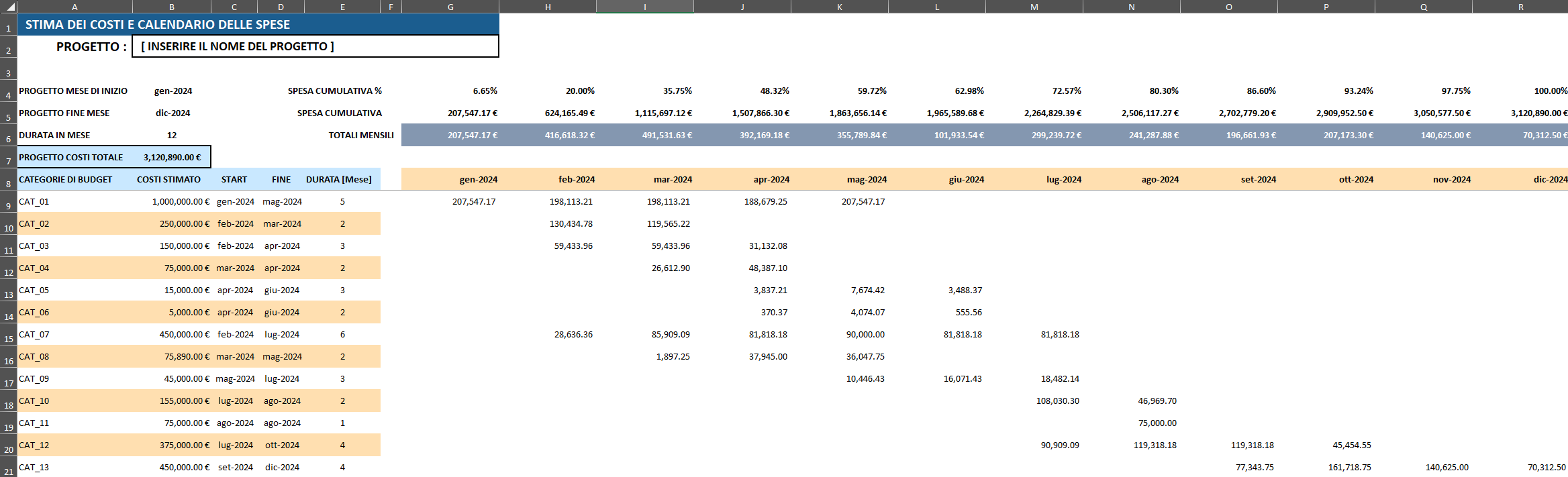
AUTO_PROSPETTO_COSTI — Cost Estimate and Expenditure Schedule — is the workbook's planning hub. Its purpose is to answer a seemingly simple question: Given a set of budget categories, each with a total cost, start date and end date, how much money should be spent in each calendar month?

The answer is not simply a lookup. The sheet distributes the cost of each category across the months it is active, weighted by the number of working days that fall within each calendar month. The result is a cost baseline broken down by time — the official plan against which actual spending will later be measured.

Here is a structure at a glance.

The sheet is organised into two zones:

• Columns A–F (rows 8 onwards): The input table. Each row defines a budget category, including its estimated cost, start date, end date, and duration in months.
• Columns G onwards: The output matrix. Each column represents a calendar month and each cell contains the estimated spend for that category in that month.

Above the data table, rows 4–7 carry contain summary rows that aggregate data across all categories, providing monthly totals, cumulative spend, and cumulative spend as a percentage of the total project budget.

The setup: Named ranges and SETUP_BASELINE

Before any calculations are performed, all master project parameters are defined in the companion sheet SETUP_BASELINE. The workbook uses named ranges to reference these values, thereby avoiding the use of hard-coded cell addresses.

The key named ranges used in this sheet are:

The category input rows (A9:F200) are not entered manually into this sheet. Instead, cell A9 contains a LET formula that pulls them live from SETUP_BASELINE:

=LET(
   cat,    (SETUP_BASELINE!B9:B200),
   ct,     (SETUP_BASELINE!C9:C200),
   inizio, (SETUP_BASELINE!D9:D200),
   fine,   (SETUP_BASELINE!E9:E200),
   durata, (SETUP_BASELINE!F9:F200),
   result, IFNA(HSTACK(cat, ct, inizio, fine, durata), ""),
   result
)

The LET function assigns a readable variable name to each source column a (e,g. cat, ct, inizio, fine, durata), and the HSTACK function assembles these into a single spilled array. IFNA(..., "") suppresses errors for empty rows at the bottom of the range.
The practical effect is that: The entire input table is populates from a single formula in A9, and updating SETUP_BASELINE is instantly reflected here.

Step 1: Generating the Month Header Row

Row 8, starting from column G, displays the first day of each project month. Cell G8 contains:

=IF(
   STARTDATE = "",
   "",
   EOMONTH(
      EDATE(STARTDATE, SEQUENCE(, MONTH(ACTUALENDDATE) - MONTH(ACTUALSTARTDATE) + 1)),
      -2
   ) + 1
)

This is a dynamic array formula that produces all month headers in a single expression:

1. SEQUENCE(, n) generates a horizontal array of integers from 1 to n, where n is the number of months between the actual start and end dates.
2. EDATE(STARTDATE, ...) offsets the start date by each integer in the sequence — one month at a time.
3. EOMONTH(..., -2) + 1 converts each offset date to the first day of its month (end of month minus 1 month, plus 1 day).

The result extends to the right across as many columns as there are month in the project. There is no need to manually extend the header row when the project duration changes, as the formula adapts automatically.

Step 2: The Core Distribution Formula (Cell G9)

This is the most complex formula in the workbook. Cell G9 calculates the estimated expenditure based on working days for every category and every month simultaneously. It is written as a combination of MAKEARRAY and LET:

=IFERROR(
  LET(
    startDates,   C9:C21,
    endDates,     D9:D21,
    taskAmounts,  B9:B21,
    totalDays,    SETUP_BASELINE!G9:G21,
    headerDates,  ANCHORARRAY(G8),

    MAKEARRAY(
      ROWS(startDates),
      COLUMNS(headerDates),
      LAMBDA(r, c,
        LET(
          taskStart,     INDEX(startDates, r),
          taskEnd,       INDEX(endDates, r),
          headerDate,    INDEX(headerDates, c),
          amount,        INDEX(taskAmounts, r),
          taskTotalDays, INDEX(totalDays, r),
          dailyRate,     IFERROR(amount / taskTotalDays, 0),

          monthStart,    IFERROR(DATE(YEAR(headerDate), MONTH(headerDate), 1),
                                 DATE(2024, c, 1)),
          monthEnd,      IFERROR(EOMONTH(monthStart, 0),
                                 EOMONTH(DATE(2024, c, 1), 0)),

          periodStart,   MAX(IFERROR(taskStart, DATE(2100,1,1)), monthStart),
          periodEnd,     MIN(IFERROR(taskEnd,   DATE(1900,1,1)), monthEnd),

          isActive,      periodStart <= periodEnd,

          monthlyDays,   IF(isActive,
                            IFERROR(NETWORKDAYS.INTL(
                              periodStart, periodEnd, 1, _DataFestivita), 0),
                            0),

          monthlyAmount, IF(monthlyDays = 0, NA(), dailyRate * monthlyDays),

          monthlyAmount
        )
      )
    )
  ),
"")

Breaking it down

Outer LET — Naming the Inputs: The outer LET gives readable names to the five input arrays (startDates, endDates, taskAmounts, totalDays), as well as to headerDates, which uses ANCHORARRAY(G8) to reference the dynamically spilled month header row.

MAKEARRAY(rows, cols, LAMBDA(r, c, ...)): MAKEARRAY is the engine. It creates a two-dimensional array, with one row for each category and one column for each month. It calls the LAMBDA function once for each cell position (r, c).

Inner LET — the per-cell calculation: Inside the LAMBDA, a second LET function defines the variables required to calculate the value of each cell:

• dailyRate = amount / taskTotalDays — The total cost of the category divided by the total number of working days across the whole project. This is the cost per working day.
• monthStart / monthEnd : the first and last day of the column's month.
• periodStart = MAX(taskStart, monthStart) :the later of the task start and the month start.
• periodEnd = MIN(taskEnd, monthEnd) : the earlier of the task end and the month end.
• isActive — true only when periodStart ≤ periodEnd, i.e. the task overlaps this month at all.
• monthlyDays — NETWORKDAYS.INTL(periodStart, periodEnd, 1, _DataFestivita) counts the working days in the overlap, excluding weekends and the public holidays listed in the feste_italia_sardegna sheet.
• monthlyAmount = dailyRate × monthlyDays.

If the task is inactive in that month, NA() is returned, which renders as a blank. The outer IFERROR(..., "") function catches any remaining errors.

Step 3: Summary Rows

Row 6 — Monthly Totals:

=BYCOL(G9:BB200, LAMBDA(col, IF(SUM(col)=0, "", SUM(col))))

BYCOL applies the LAMBDA function to each column in of the data range, adding up all the values in the Categorycolumn for that month. Empty months return "".

Row 5 — Cumulative Spend:

=BYCOL(G6:BB6, LAMBDA(col, IF(col="", "", SUM(col:G$6))))

This accumulates for each monthly total from column G up to and including the current column. The anchor G$6 ensures that the running sum always starts from the first month.

Row 4 — Cumulative Spend %:

=BYCOL(G5:BB5, LAMBDA(col, IF(col="", "", col / TOTALCOST)))

It divides each cumulative figure by the named range TOTALCOST to produce the S-curve percentage values used in the chart sheet.

Why NETWORKDAYS.INTL Matters

Using working-day weighting rather than calendar-day weighting is important for controlling project costs. For example, a category running from 29 January to 3 February spans two calendar months, but nearly all of its cost accrues in January in terms of working days. Calendar-day proration would therefore misstate the baseline. However, by using the NETWORKDAYS.INTL function with the _DataFestivita holiday list, the model correctly accounts for public holidays. For example, a month containing a cluster of Italian bank holidays will have fewer chargeable days and therefore a lower allocated cost.

Key Takeaways

• The entire input table is populated by a single LET/HSTACK formula in A9, driven by SETUP_BASELINE.
• The month header row (G8) is a dynamic array that expands automatically as the project duration changes.
• The distribution matrix (G9 onwards) is computed by a single MAKEARRAY/LAMBDA/LET formula which iterates over every row-column intersection, eliminating the need for any helper columns.
• Cost allocation is based on working days, not calendar days, using a dedicated holiday calendar.
• BYCOL/LAMBDA patterns in the summary rows keep aggregation formulas lean and self-extending.

Visualisations (this article)

Diagram 1 — Formula architecture: from SETUP_BASELINE to the distribution matrix. Shows the three-layer structure: named range inputs feeding the LET/HSTACK formula in A9, which feeds the MAKEARRAY engine in G9, which produces the output matrix; the BYCOL summary rows sit below.

Diagram 2 — Inside the MAKEARRAY cell: how a single monthly spend value is computed. Traces the three inputs (daily rate, month boundaries, overlap period) into NETWORKDAYS.INTL, and from there to the final monthly amount.

Read the next part of this series: Data from a ledger flows into a time-structured actual cost matrix. (Cost-based expenditure plan, Part 03)

The following article in the series has already been published: Before the formulas, the architecture (Cost Baseline Expenditure Schedule Part 01)